BGM：《Aldnoah Zero》ED1
歌词混好几种语言

参考《Hands-On Machine Learning with Scikit-Learn and TensorFlow(2017)》Chap14
《Hands-On Machine Learning with Scikit-Learn and TensorFlow》笔记

【占坑待填】
Handson ML对RNN的介绍比较简略，先占着坑

Basic RNNs的tensorflow实现

• Jupyter - Static Unrolling Through Time(Plain)
  底层操作实现的静态展开
• Jupyter - Unrolling Through Time(High-level_API)
  高层操作实现的静态展开和动态展开
• Jupyter - Handling Variable Length Sequences
  处理变长的输入输出，另外还有一种办法，参见5.2 机器翻译（Encoder-Decoder）

训练RNN（BackproPagation Through Time, BPTT）

一般将RNN按时间展开，然后使用常规的反向传播进行训练；
如下图所示：

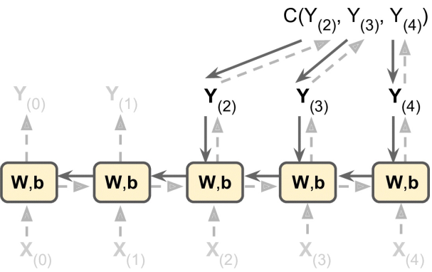
注意这里损失函数 C(·) 是由最后几个输出计算得到的，而不是最后一个输出！

序列分类器

类似CNN做MNIST分类器，RNN也可以实现手写数字的识别；
按照《Handson-ML》，准确率也可以达到98%以上

预测时间序列

比如股价预测——
随机截取一些连续的20个时间点的股价作为mini-batch，并且右移1个时间点作为标注；
即训练一个预测下一个时间点的股价的模型；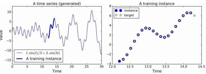

按前述直接用动态展开的BasicRNNCell组成的RNN网络——

n_steps = 20
n_inputs = 1
n_neurons = 100
n_outputs = 1

X = tf.placeholder(tf.float32, [None, n_steps, n_inputs])
y = tf.placeholder(tf.float32, [None, n_steps, n_outputs])
cell = tf.contrib.rnn.BasicRNNCell(num_units=n_neurons, activation=tf.nn.relu)
outputs, states = tf.nn.dynamic_rnn(cell, X, dtype=tf.float32)

但是此时的网络输出outputs是一个包含100元素（n_neurons=100）的向量，
而我们需要的只是一个元素，即使下一时刻的预测值，最简单的思路是对cell进行包装：
其实就是在BasicRNNCell之后再加一个fully connected层（无激活函数）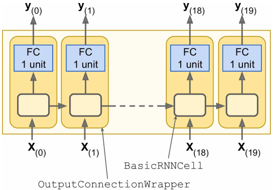

具体实现——

# [...]
basic_cell = tf.contrib.rnn.BasicRNNCell(num_units=n_neurons, activation=tf.nn.relu)
cell = tf.contrib.rnn.OutputProjectionWrapper(basic_cell, output_size=n_outputs)
outputs, states = tf.nn.dynamic_rnn(cell, X, dtype=tf.float32)

此时的outputs就是一个单元素的输出啦~
尽管OutputProjectionWrapper可以解决这一问题，但每一步的神经元输出都需要过一层FC，效率不是很高；
更好的办法是（只需要过一次FC）：

1. 将RNN的输出从 [batch_size, n_steps, n_neurons] 重整为 [batch_size * n_steps, n_neurons]；
2. 再通过一个fully connected整合成 [batch_size * n_steps, n_outputs] 大小的输出；
3. 最后展开成 [batch_size, n_steps, n_outputs] 大小的最终输出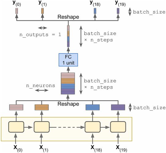
   

具体实现——

# [...]
basic_cell = tf.contrib.rnn.BasicRNNCell(num_units=n_neurons, activation=tf.nn.relu)
rnn_outputs, states = tf.nn.dynamic_rnn(basic_cell, X, dtype=tf.float32)

# 将RNN的输出从 [batch_size, n_steps, n_neurons] 重整为 [batch_size * n_steps, n_neurons]
stacked_rnn_outputs = tf.reshape(rnn_outputs, [-1, n_neurons])
# 通过一个fully connected整合成 [batch_size * n_steps, n_outputs] 大小的输出
stacked_outputs = fully_connected(stacked_rnn_outputs, n_outputs, activation_fn=None)
# 最后展开成 [batch_size, n_steps, n_outputs] 大小的最终输出
outputs = tf.reshape(stacked_outputs, [-1, n_steps, n_outputs])

深层RNN

直接堆叠RNN就可以得到一个深层的RNN——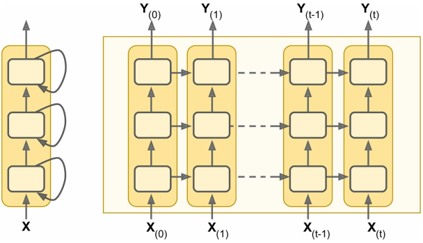

具体实现——
借助 tf.contrib.rnn.MultiRNNCell() 可以将多个RNN堆叠起来

n_neurons = 100
n_layers = 3

basic_cell = tf.contrib.rnn.BasicRNNCell(num_units=n_neurons)
multi_layer_cell = tf.contrib.rnn.MultiRNNCell([basic_cell] * n_layers)
outputs, states = tf.nn.dynamic_rnn(multi_layer_cell, X, dtype=tf.float32)

此时 states 是一个元组，每个元素都是每一层对应的大小为 [batch_size, n_neurons] 的Tensor；
如果为 MultiRNNCell 指定参数 state_is_tuple=False ，那么 states 就只是一个 [batch_size, n_layers * n_neurons] 大小的Tensor；

分布式训练

……暂略……

使用Dropout

如果只是在RNN层之前或者之后，可以直接添加Dropout层【可以参见正则化技术 - Dropout】；
但如果是在RNN层与RNN层之间添加Dropout，就必须使用 DropoutWrapper：

keep_prob = 0.5

cell = tf.contrib.rnn.BasicRNNCell(num_units=n_neurons)
# 用DropoutWrapper包装BasicRNNCell
# ... input_keep_prob参数是输入前dropout层的keep_prob（不指定则步添加dropout）
# ... 相应的还有output_keep_prob参数
cell_drop = tf.contrib.rnn.DropoutWrapper(cell, input_keep_prob=keep_prob)
# 直接堆叠若干个RNN层，层与层之间不能直接使用Dropout层
multi_layer_cell = tf.contrib.rnn.MultiRNNCell([cell_drop] * n_layers)
rnn_outputs, states = tf.nn.dynamic_rnn(multi_layer_cell, X, dtype=tf.float32)

然而头疼的是，DropoutWrapper 并不支持 is_training 参数，也就是说，它在预测是依旧存在dropout层；
解决方法有两种——

1. 自己重写一个支持 is_training 参数的 DropoutWrapper 类（什么鬼设定）

2. 针对训练和预测构建不同的计算图，具体如下：

    import sys
    is_training = (sys.argv[-1] == "train")
   
    X = tf.placeholder(tf.float32, [None, n_steps, n_inputs])
    y = tf.placeholder(tf.float32, [None, n_steps, n_outputs])
   
    cell = tf.contrib.rnn.BasicRNNCell(num_units=n_neurons)
    if is_training:     # 如果是训练，则用DropoutWrapper包装；如果是预测就拉倒
        cell = tf.contrib.rnn.DropoutWrapper(cell, input_keep_prob=keep_prob)
    multi_layer_cell = tf.contrib.rnn.MultiRNNCell([cell] * n_layers)
    rnn_outputs, states = tf.nn.dynamic_rnn(multi_layer_cell, X, dtype=tf.float32)
    # [...] build the rest of the graph
    init = tf.global_variables_initializer()
    saver = tf.train.Saver()
   
    with tf.Session() as sess:
        if is_training:     # 如果是训练，那就执行初始化器并进行训练
            init.run()
            for iteration in range(n_iterations):
                # [...] # train the model
                save_path = saver.save(sess, "/tmp/my_model.ckpt")
        else:   # 如果是预测，那就直接载入模型并使用
            saver.restore(sess, "/tmp/my_model.ckpt")
            # [...] # use the model
   

长期依赖问题

梯度消失与梯度爆炸 所述技术对RNN也是有效的；
但是使用这些技术之后，随着时间步增多，训练将变得十分缓慢；
最简单粗暴的解决方法是缩短时间步，但如此一来RNN忽略比较遥远的过去，也即存在长期依赖的问题；
为了解决这一问题，LSTM出现啦！

LSTM

论文：
【起源】：Long Short-Term Memory(2006)
【改进】：

1. LONG SHORT-TERM MEMORY BASED RECURRENT NEURAL NETWORK ARCHITECTURES FOR LARGE VOCABULARY SPEECH RECOGNITION(2014)
2. RECURRENT NEURAL NETWORK REGULARIZATION(2015)
3. Recurrent Nets that Time and Count(2000) 【提出peephole connection】
4. Learning Phrase Representations using RNN Encoder–Decoder for Statistical Machine Translation(2014) 【提出GRU和Encoder-Decoder架构】
   其他：Understanding LSTM Networks(2015)

tensorflow中的使用：
直接将先前的 tf.contrib.rnn.BasicRNNCell 替换为 tf.contrib.rnn.BasicLSTMCell 即可；
区别在于，BasicLSTMCell 的states包含两个向量，如果要合并在一起的话可以指定参数 state_is_tuple=False；
如果要使用变种的LSTM，则使用 tf.contrib.rnn.LSTMCell：
比如使用带peephole connection的LSTM，则指定参数 use_peepholes=True

tf.contrib.rnn.LSTMCell(num_units=n_neurons, use_peepholes=True)

应用

The Unreasonable Effectiveness of Recurrent Neural Networks(2015) 一问介绍了RNN的一些应用；

接下来只介绍RNN在自然语言处理（NLP）上的两个应用

词嵌入

参考：

1. Tensorflow Tutorial - Word2Vec 或 中文的字词的向量表示
2. Deep Learning, NLP, and Representations(2014)
3. Word Embeddings in 2017: Trends and future directions(2017)

词表示的方式：

1. 独热码：稀疏表示
2. 顺序编码：稠密表示
3. 词嵌入：前两者的折中，而且可以通过训练，使得两个词的距离表示它们的相似程度

tensorflow实现：

vocabulary_size = 50000
embedding_size = 150

# 创建一个待训练的词向量变量
embeddings = tf.Variable( tf.random_uniform([vocabulary_size, embedding_size], -1.0, 1.0) )
# 占位符，输入单词的顺序编码
train_inputs = tf.placeholder(tf.int32, shape=[None])
# 用embedding_lookup获取对应单词的顺序编码对应的词向量表示
embed = tf.nn.embedding_lookup(embeddings, train_inputs)

# [...] 投喂语料库训练出合适的词向量
# 投喂前需要预处理语料库，比如将一些未知的单词都置为<UNK>、将链接都置为<URL>

当然，也可以直接下载已经训练好的词向量载入给 embedding 然后直接使用；

机器翻译（Encoder-Decoder）

参考：Tensorflow Tutorial - Seq2Seq 【代码】

训练时：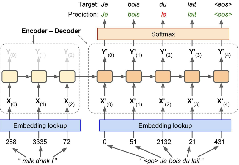

• 源语句投喂给Encoder，注意应该使第一个单词最先进入Decoder
• 目标语句投喂给Decoder
• Decoder对每个时间步产生一个评分并交由Softmax层得到单词的输出概率

预测时：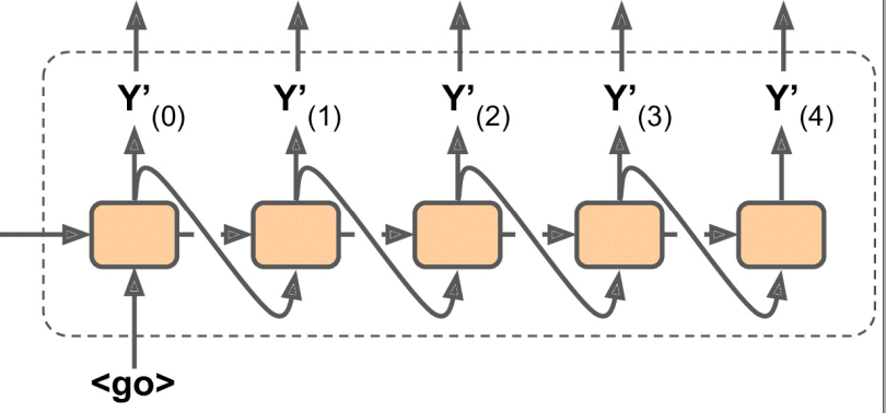

Google - Seq2Seq项目的特别之处：

1. 独特的处理变长序列的方式
   前述提到用 sequence_length参数+静态展开 或 动态展开 的方式来处理变长序列；
   而Seq2Seq采用另一种方式——
   先将语句根据不同长度段分别放入不同的桶中（比如有接收长度为1~6的语句桶、接收长度为7~12的语句桶）；
   再用符号 <pad> 将桶内的语句填充到同一规格（比如I drink milk <eos>被填充为I drink milk <eos> <pad> <pad>）；
   （注意，源语句在前面填充符号，目标语句在末尾填充符号）
   然后用一个 target_weights 向量表征每个单词的权重（比如I drink milk <eos> <pad> <pad>的权重为[1,1,1,1,0,0]）；
   这样，当损失函数与 target_weights 向量相乘时，<pad> 就被忽略了；
2. 使用Sampled Softmax技术
   论文：On Using Very Large Target Vocabulary for Neural Machine Translation
   当输出字典非常大（比如50000）时，Decoder将产生50000维的向量，使得计算softmax函数时变得非常复杂；
   为了避免这个问题，可以使Decoder输出小得多的向量（如1000维），然后用采样技术来评估损失；
   这在tensorflow中可以借助函数 sampled_softmax_loss() 实现
3. 使用注意力机制
   论文：Show, Attend and Tell: Neural Image Caption Generation with Visual Attention
4. Seq2Seq使用了 tf.nn.legacy_seq2seq 模块，模块中包含了各种各样的Encoder-Decoder模型
   比如 embedding_rnn_seq2seq() 函数创建一个与前述机器翻译训练时的图中相同的模型